We all must have manually formatted our excel spreadsheet at some point in time either for creating a border or highlighting a cell or some other basic formatting features. However there is a better way of formatting your excel sheets without even putting any manual effort every time you need something formatted in a specific manner. I’m talking about CONDITIONAL FORMATTING. Let's see how it's done.
Today you will see how we can use conditional formatting to automate those boring formatting tasks which required your manual intervention earlier.

Data Used
https://docs.google.com/spreadsheets/d/1JJswJgMKU2EMHxwErPucDC1vaiPe_xnLrgjjbpN4XLo/edit?usp=sharing
Format cells based on a cell value
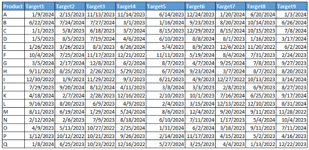
Let's kick off things with a simple formatting task where you want to color a cell if it has a certain value. I have a simple table below which shows Sales figures for a few products across various countries.
Task :
Highlight cells in Country column if the value is Mexico

Steps to apply formula based conditional formatting
1. Select the cells that you want to color. So in this case select all the cells in Country column

2. Click on New Rule (Home > Conditional Formatting)

3. Click on the last option i.e. Use a formula to determine which cells to format

4. Enter the following formula in the Formula bar like below. This formula tells excel to format the cells where value equals “Mexico”.
(assuming country column in your excel sheet is in D column)
=$D3="Mexico" |
5. Click on Format button & use the color of your choice and press OK
Please note how only the “$” dollar sign is in front of “D” but not before 3. That is because we want excel to drag the same formula


Format cells if a date is falling within a dynamic range
Now lets see another scenario where we will use a bit more complex formula than before but its variation can be applied in multiple problem statements.
Task :
Highlight cells if a Sales Target date is falling within 30 days from today
Steps to apply formula based conditional formatting
1. Following the same steps like before, select the range of cells where you want to apply conditional formatting and then go to Home > Conditional Formatting > New Rule

2. Enter below formula in the formula bar & select desired color for formatting. Here we are using a combination of AND operator and our conditions because we want excel to check if the value is greater than or equal to TODAY AND less than 30 days from today.
=AND(C3>=Today(),C3<Today()+30) |
Please note that this time we have not used “$” dollar sign anywhere because the range is expanded in multiple columns & rows.


Search box using Conditional Formatting
Lets become a bit more creative and create a search function which gives you the control to format cells based on the value you enter into the SEARCH box.
Task : Highlight cells values which matches the search criteria entered by user in a cell

Steps to apply formula based conditional formatting
1. Following the same steps like before, select the range of cells where you want to apply conditional formatting and then go to Home > Conditional Formatting > New Rule

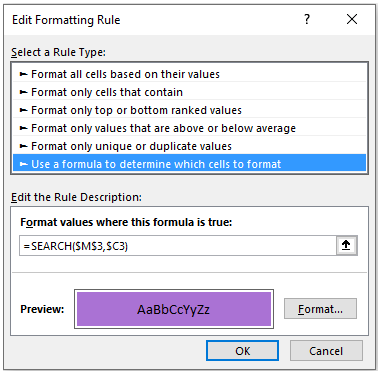
2. Enter the below formula into the formula bar & select the desired color. This formula is instructing excel to search the value entered by the user in cell $M$3 against the desired range i.e. C column
As we learned earlier, no dollar sign before row number i.e. 3 since we want the formula to be extended to the entire range.
=SEARCH($M$3,$C3) |

Now you can apply this knowledge in more creative ways to solve multiple problem statements. For example we can use OR statements, apply different formatting styles like fonts, borders etc.
Comments