Data transformation is one of the key steps in the Data Analytics world but often it is overlooked which leads to huge amounts of rework in your analysis. Every data analyst or data engineer should spend a good amount of time understanding the data & then transforming it in a way that makes absolute sense to the business objective.
Now that we have established the importance of Data Transformation, let me introduce you to today’s topic which is utilizing the amazing tools included within Excel Power Query to transform any data with relative ease. Let's see how it's done!

Data Used
This a list of various cars produced within a country and few specifications related to its Manufacturing, Fuel type, Owner Type etc.

Requirements
Create 2 different dataset from this master table
Table 1 -
Summary table with 2 columns, i.e. Name & Avg Selling Price
Replace “Maruti” with “Maruti Suzuki”
Table 2 -
Data of cars manufactured in 2020, however Car Names in Column while Selling Price & KM driven in Rows
Rename the Column Header name to “Car Name” in 2nd table
Data Loading into Power Query
Select the data range in your excel worksheet & then Click on Data >> From Table/Range

If your data has a header then select the checkbox and press OK. This will open the Power Query Editor

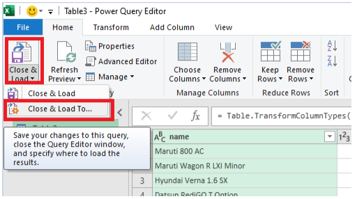
Finally Close & LoadTo >> Only Create Connection we are doing this because this is not our final output & we don't want this table to take any space in our excel file.

Requirement #1
Summary table with 2 columns, i.e. Name & Avg Selling Price
Replace “Maruti” with “Maruti Suzuki”
Go back to the Power Query Editor by double clicking on the connection

Create a Duplicate of the main table by right clicking on the main table & then selecting Duplicate. Here we are just creating a duplicate of the original table to create our 1st requirement table

Select the Name column from the table since we want to summarize our data based on the Name column. Then click on Group By

Give the column a new name and then
select Average from the Operation dropdown
Selling_Price from the Column dropdown. Press OK

Finally Select Name column and then click on Replace Values. And then Enter Maruti in the Value to Find section and enter Maruti Suzuki in Replace With section. Press OK


That's it, the 1st requirement is completed.
Requirement #2
Data of cars manufactured in 2020, however Car Names in Column while Selling Price & KM driven in Rows
Rename the Column Header name to “Car Name” in 2nd table
Create another duplicate table of the original table, similar to what we did for the 1st requirement
Select the year column and in the filter apply a filter for 2020 and press OK

Select column Name, Selling Price & KM Driven. And then click on Remove Other Columns

Now this is an IMPORTANT STEP. If you don't follow this then your data will will not have Row Categories, instead it will look like below

Select “Use Header as First Row”

Now click on Transpose
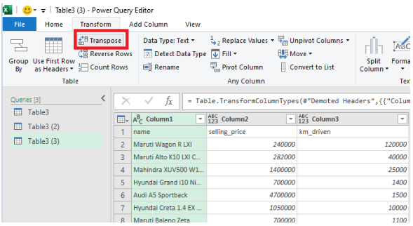
Click on “Use First Row as Header”

For the final step, right click on the column header “name” and then click on rename to name the header as “Car Name”

That's it, we are done. Now we can click on “Close & Load”. Since these 2 tables were the duplicate of the master table, excel will treat this as a connection too.
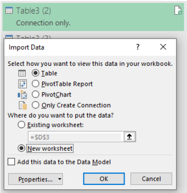
So if you want to input the data in the sheet then
Right click on the query in the sheet and select “Load To” and then select Table & New Worksheet from the radio buttons. Press Ok
Comments