Wildcards are simply awesome because it has the potential to reduce your analysis efforts to just seconds. It has been a secret recipe for many excel users while working on complex data analysis projects or building interactive dashboards.
Today we will see different types of wildcards in excel and it usages in multiple scenarios. Also I will share a quick tip for using Wildcard when you are designing a dashboard and providing the user with dropdown selection functionality. Let's see how it's done!

Dataset Used
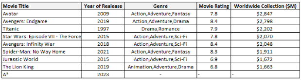
I have taken here a small snippet of the actual dataset to help you understand the concept in a digestible chunk. Also I added the last row item to explain a specific concept.
Types of Wildcards & its usage
Wildcards can only be used on characters, it will not work on numbers
Asterisk (*)
Start With : Let say you want to find out the count of movies that start with the character “a”, and can have any number of characters after that. In this case you can use below formula : =COUNTIF(I5:I12,"a*")
End With : Now we want the sum of Gross revenue of movies that end with the word “r”, but can have any number of characters in front of that. In this case we will have to input “*” in front of r =SUMIF(I5:I12,"*r",M5:M12)
Contains : Now we have to find out the count of movies which are in the “Drama” genre. So we will have to use “*” both in front & back of the word “Drama”, like below =COUNTIF(K5:K12,"*Drama*")
Select All : This is a quick tip while you are designing a dashboard and want users to have an option of “All” in any kind of dropdown feature. Let say you have created a dropdown using Data Validation in a cell and want the user to see Gross Revenue information whenever they select a movie name from the dropdown, however you also want the user to have an option to see total Gross Revenue of all movies. In this case add a new item in the validation list as “All” and then use below formula =IF(F6="All", SUMIF(I5:I12,"*",M5:M12), SUMIF(I5:I12,F6,M5:M12)) This will give you the total Gross Revenue when user selects “All” in cell F6
Question Mark (?)
Count Characters : When you want to run a formula when a certain number of characters is found in a cell then we can use “?”. For example, I have to find out the count of movies which has exactly 6 characters, so I can use the below formula which has 6 question marks =COUNTIF(I5:I12,"??????") Similarly if I want to find any number of characters, I can use that number of question marks in the formula.
Usage of Question Mark with Asterisk : Suppose I want to find out the count of movies which has 9 character in front and then any number of characters after that, then I can use below formula =COUNTIF(I5:I12,"?????????*")
Tilde (~)
Nullify Wildcards : Now comes the concept for which I inserted that additional row item in the raw data. Suppose now you want to apply a Vlookup formula and find out movie by the name of “A*”, then in this case normal Vlookup will not fetch the correct information because excel will treat “*” after the “A” as a wildcard but in this case we want to treat the value as it is, so we can use “~” to nullify the wildcard =VLOOKUP("a~*",I5:M13,2,0)
Comentários