No matter how we analyze our data, formatting remains a key part of the activity because it helps us clearly view the data in our desired format. This can be in the form of Text, Date, Number or any color.
By default excel gives us many formatting options like date, currency, accounting etc. which are very useful, but today we are going to especially focus on creating custom formatting and the rules that we need to keep in mind while creating the same. Let's go!

Data Used
The data represent the sales of few products with its selling price and the Profit/Loss from the same

Requirements
All number values should be formatted with “Thousand separators” & 2 Decimal Points
Format the negative value in red color
If we have any 0 values then show “-”
And if accidentally someone entered a text value then show “Invalid” in blue color
Understanding the Structure of Custom Formatting
In order to master custom formatting we need to understand its structure. It does not change the underlying data but It gives you a unique control over your data by transforming visual representation of your values.
Most of us don’t realize this but Custom Formatting is divided into 4 sections with each separated by a semicolon (;), performing a specific role.

First Section - This defines all Positive values in your cell or range i.e. how do you want to display any positive values
Second Section - This defines all Negative values and how you want to show them
Third Section - If you have any 0 values then this is where we define its formatting
Fourth Section - The last section is for formatting any Text values in your data
Now remember that all sections of the custom formatting are not required while you create your formatting.
If you input just the 1st section then it applies to all Positive, Negative & Zero values
If you input 1st & 2nd section then the 1st one applies to all Positive & Zero values, while the 2nd applies to all Negative values
Text formatting is only applied if you explicitly write the 4th section
Number & Text Code

These are a few number and text codes that are used for formatting. As you see each has a specific function which can be used in combination with each other to derive very interesting results. Above table highlights a few of those combinations with examples for each.
Let’s complete the requirements now
Now that we have seen all basic rules & codes which are used in Custom Formatting, let us now dive into our problem statement for today
#1 : All number values should be formatted with “Thousand separators” & 2 Decimal Points
#2 : Format negative values in red color
#3 : Zero values to be shown as “-”
#4 : Text value to be shown as “Invalid” in blue color
Select the entire range of cells where you want to apply the formatting

Press Ctrl + 1 on your keyboard
Now in the new prompt window, select Custom and remove the default value from the Type section
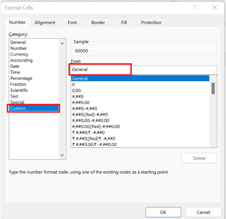
Now in the Type section enter below code
#,###.00 ;[Red] -#,###.00 ; "-" ;[Blue] "Invalid"
Let’s understand the format code now
As we understood earlier, custom formatting has 4 sections and each section is separated by a semicolon (;). Let us understand each section individually now
#,###.00 : This section is for positive values. We have used # sign to represent significant value along with a thousand separators. While adding 00 after decimal for instructing excel to display 2 decimal points at all times.
[Red] -#,###.00 : This section is for negative values so apart from the same format code as above we have added “-” negative sign. Also since we want to add a red color to the text, we have given the color code inside [] square brackets.
"-" : This section is for formatting Zero values, so in this case we have simply given “-”, so that it displays the same when a zero value is entered
[Blue] "Invalid" : The final section is for text, so we have first given it a color code and since we don't want to display the actual text, we have not used @ , instead we have given the text value we wanted i.e. “Invalid”.
Comments