Introduction to Churn Analysis
In today’s competitive business environment, retaining customers is crucial for long-term success. Churn analysis is a key technique used to understand and reduce this customer attrition. It involves examining customer data to identify patterns and reasons behind customer departures. By using advanced data analytics and machine learning, businesses can predict which customers are at risk of leaving and understand the factors driving their decisions. This knowledge allows companies to take proactive steps to improve customer satisfaction and loyalty.
Data & Other Resources Used
Colors used
#4A44F2, #9B9FF2, #F2F2F2, #A0D1FF
Who is the Target Audience
Although this project focuses on churn analysis for a telecom firm, the techniques and insights are applicable across various industries. From retail and finance to healthcare and beyond, any business that values customer retention can benefit from churn analysis. We will explore the methods, tools, and best practices for reducing churn and improving customer loyalty, transforming data into actionable insights for sustained success.
Project Target
Create an entire ETL process in a database & a Power BI dashboard to utilize the Customer Data and achieve below goals:
- Visualize & Analyse Customer Data at below levels
- Demographic
- Geographic
- Payment & Account Info
- Services
- Study Churner Profile & Identify Areas for Implementing Marketing Campaigns
- Identify a Method to Predict Future Churners
Metrics Required
- Total Customers
- Total Churn & Churn Rate
- New Joiners
STEP 1 – ETL Process in SQL Server
So the first step in churn analysis is to load the data from our source file. For this purpose we will be using Microsoft SQL server because it is a widely used solution across the industry and also because a full-fledged Database System is better at handling recurring data loads and maintaining data integrity compared to an excel file.
Download SSMS
In order for us to run our sql queries Microsoft provides us with GUI interface which is known as SQL Server Management Studio. You can download the latest version from the link provided below.
Creating Database
After installation, you will land on the following screen. Do remember to copy paste the server name somewhere because we will need this at a later stage. Also enable the checkbox which says “Trust Server Certificate” and then click on Connect
Once connected, click on NEW QUERY button at the top ribbon and then write below query. This will create a new Database named db_Churn
CREATE DATABASE db_Churn
Import csv into SQL server staging table – Import Wizard
Right click on the newly created database in the explorer window and then go to
Task >> Import >> Flat file >> Browse CSV file
Remember to add customerId as primary key and allow nulls for all remaining columns. This is done to avoid any errors while data load. Also make sure to change the datatype where it say Bit to Varchar(50). We are doing this because while using import wizard I faced issues with the BIT data type, however Varchar(50) works fine.
Data Exploration – Check Distinct Values
SELECT Gender, Count(Gender) as TotalCount,
Count(Gender)  1.0 / (Select Count() from stg_Churn)  as Percentage
from stg_Churn
Group by Gender
SELECT Contract, Count(Contract) as TotalCount,
Count(Contract)  1.0 / (Select Count() from stg_Churn)  as Percentage
from stg_Churn
Group by Contract
SELECT Customer_Status, Count(Customer_Status) as TotalCount, Sum(Total_Revenue) as TotalRev,
Sum(Total_Revenue) / (Select sum(Total_Revenue) from stg_Churn) * 100  as RevPercentage
from stg_Churn
Group by Customer_Status
SELECT State, Count(State) as TotalCount,
Count(State)  1.0 / (Select Count() from stg_Churn)  as Percentage
from stg_Churn
Group by State
Order by Percentage desc
Data Exploration – Check Nulls
SELECT
    SUM(CASE WHEN Customer_ID IS NULL THEN 1 ELSE 0 END) AS Customer_ID_Null_Count,

    SUM(CASE WHEN Gender IS NULL THEN 1 ELSE 0 END) AS Gender_Null_Count,

    SUM(CASE WHEN Age IS NULL THEN 1 ELSE 0 END) AS Age_Null_Count,

    SUM(CASE WHEN Married IS NULL THEN 1 ELSE 0 END) AS Married_Null_Count,

    SUM(CASE WHEN State IS NULL THEN 1 ELSE 0 END) AS State_Null_Count,

    SUM(CASE WHEN Number_of_Referrals IS NULL THEN 1 ELSE 0 END) AS Number_of_Referrals_Null_Count,

    SUM(CASE WHEN Tenure_in_Months IS NULL THEN 1 ELSE 0 END) AS Tenure_in_Months_Null_Count,

    SUM(CASE WHEN Value_Deal IS NULL THEN 1 ELSE 0 END) AS Value_Deal_Null_Count,

    SUM(CASE WHEN Phone_Service IS NULL THEN 1 ELSE 0 END) AS Phone_Service_Null_Count,

    SUM(CASE WHEN Multiple_Lines IS NULL THEN 1 ELSE 0 END) AS Multiple_Lines_Null_Count,

    SUM(CASE WHEN Internet_Service IS NULL THEN 1 ELSE 0 END) AS Internet_Service_Null_Count,

    SUM(CASE WHEN Internet_Type IS NULL THEN 1 ELSE 0 END) AS Internet_Type_Null_Count,

    SUM(CASE WHEN Online_Security IS NULL THEN 1 ELSE 0 END) AS Online_Security_Null_Count,

    SUM(CASE WHEN Online_Backup IS NULL THEN 1 ELSE 0 END) AS Online_Backup_Null_Count,

    SUM(CASE WHEN Device_Protection_Plan IS NULL THEN 1 ELSE 0 END) AS Device_Protection_Plan_Null_Count,

    SUM(CASE WHEN Premium_Support IS NULL THEN 1 ELSE 0 END) AS Premium_Support_Null_Count,

    SUM(CASE WHEN Streaming_TV IS NULL THEN 1 ELSE 0 END) AS Streaming_TV_Null_Count,

    SUM(CASE WHEN Streaming_Movies IS NULL THEN 1 ELSE 0 END) AS Streaming_Movies_Null_Count,

    SUM(CASE WHEN Streaming_Music IS NULL THEN 1 ELSE 0 END) AS Streaming_Music_Null_Count,

    SUM(CASE WHEN Unlimited_Data IS NULL THEN 1 ELSE 0 END) AS Unlimited_Data_Null_Count,

    SUM(CASE WHEN Contract IS NULL THEN 1 ELSE 0 END) AS Contract_Null_Count,

    SUM(CASE WHEN Paperless_Billing IS NULL THEN 1 ELSE 0 END) AS Paperless_Billing_Null_Count,

    SUM(CASE WHEN Payment_Method IS NULL THEN 1 ELSE 0 END) AS Payment_Method_Null_Count,

    SUM(CASE WHEN Monthly_Charge IS NULL THEN 1 ELSE 0 END) AS Monthly_Charge_Null_Count,

    SUM(CASE WHEN Total_Charges IS NULL THEN 1 ELSE 0 END) AS Total_Charges_Null_Count,

    SUM(CASE WHEN Total_Refunds IS NULL THEN 1 ELSE 0 END) AS Total_Refunds_Null_Count,

    SUM(CASE WHEN Total_Extra_Data_Charges IS NULL THEN 1 ELSE 0 END) AS Total_Extra_Data_Charges_Null_Count,

    SUM(CASE WHEN Total_Long_Distance_Charges IS NULL THEN 1 ELSE 0 END) AS Total_Long_Distance_Charges_Null_Count,

    SUM(CASE WHEN Total_Revenue IS NULL THEN 1 ELSE 0 END) AS Total_Revenue_Null_Count,

    SUM(CASE WHEN Customer_Status IS NULL THEN 1 ELSE 0 END) AS Customer_Status_Null_Count,

    SUM(CASE WHEN Churn_Category IS NULL THEN 1 ELSE 0 END) AS Churn_Category_Null_Count,

    SUM(CASE WHEN Churn_Reason IS NULL THEN 1 ELSE 0 END) AS Churn_Reason_Null_Count

FROM stg_Churn;
Remove null and insert the new data into Prod table
SELECT
    Customer_ID,

    Gender,

    Age,

    Married,

    State,

    Number_of_Referrals,

    Tenure_in_Months,

    ISNULL(Value_Deal, 'None') AS Value_Deal,

    Phone_Service,

    ISNULL(Multiple_Lines, 'No') As Multiple_Lines,

    Internet_Service,

    ISNULL(Internet_Type, 'None') AS Internet_Type,

    ISNULL(Online_Security, 'No') AS Online_Security,

    ISNULL(Online_Backup, 'No') AS Online_Backup,

    ISNULL(Device_Protection_Plan, 'No') AS Device_Protection_Plan,

    ISNULL(Premium_Support, 'No') AS Premium_Support,

    ISNULL(Streaming_TV, 'No') AS Streaming_TV,

    ISNULL(Streaming_Movies, 'No') AS Streaming_Movies,

    ISNULL(Streaming_Music, 'No') AS Streaming_Music,

    ISNULL(Unlimited_Data, 'No') AS Unlimited_Data,

    Contract,

    Paperless_Billing,

    Payment_Method,

    Monthly_Charge,

    Total_Charges,

    Total_Refunds,

    Total_Extra_Data_Charges,

    Total_Long_Distance_Charges,

    Total_Revenue,

    Customer_Status,

    ISNULL(Churn_Category, 'Others') AS Churn_Category,

    ISNULL(Churn_Reason , 'Others') AS Churn_Reason


INTO [db_Churn].[dbo].[prod_Churn]

FROM [db_Churn].[dbo].[stg_Churn];
Create View for Power BI
Create View vw_ChurnData as
    select * from prod_Churn where Customer_Status In ('Churned', 'Stayed')
Create View vw_JoinData as
    select * from prod_Churn where Customer_Status = 'Joined'
STEP 2 – Power BI Transform
Add a new column in prod_Churn
1. Churn Status = if [Customer_Status] = “Churned” then 1 else 0
2. Change Churn Status data type to numbers
3. Monthly Charge Range = if [Monthly_Charge] < 20 then “< 20” else if [Monthly_Charge] < 50 then “20-50” else if [Monthly_Charge] < 100 then “50-100” else “> 100”
Create a New Table Reference for mapping_AgeGrp
1. Keep only Age column and remove duplicates
2. Age Group = if [Age] < 20 then “< 20” else if [Age] < 36 then “20 – 35” else if [Age] < 51 then “36 – 50” else “> 50”
3. AgeGrpSorting = if [Age Group] = “< 20” then 1 else if [Age Group] = “20 – 35” then 2 else if [Age Group] = “36 – 50” then 3 else 4
4. Change data type of AgeGrpSorting to Numbers
Create a new table reference for mapping_TenureGrp
1. Keep only Tenure_in_Months and remove duplicates
2. Tenure Group = if [Tenure_in_Months] < 6 then “< 6 Months” else if [Tenure_in_Months] < 12 then “6-12 Months” else if [Tenure_in_Months] < 18 then “12-18 Months” else if [Tenure_in_Months] < 24 then “18-24 Months” else “>= 24 Months”
3. TenureGrpSorting = if [Tenure_in_Months] = “< 6 Months” then 1 else if [Tenure_in_Months] = “6-12 Months” then 2 else if [Tenure_in_Months] = “12-18 Months” then 3 else if [Tenure_in_Months] = “18-24 Months ” then 4 else 5
4. Change data type of TenureGrpSorting to Numbers
Create a new table reference for prod_Services
1. Unpivot services columns
2. Rename Column – Attribute >> Services & Value >> Status
STEP 3 – Power BI Measure
Total Customers = Count(prod_Churn[Customer_ID])
New Joiners = CALCULATE(COUNT(prod_Churn[Customer_ID]), prod_Churn[Customer_Status] = “Joined”)
Total Churn = SUM(prod_Churn[Churn Status])
Churn Rate = [Total Churn] / [Total Customers]
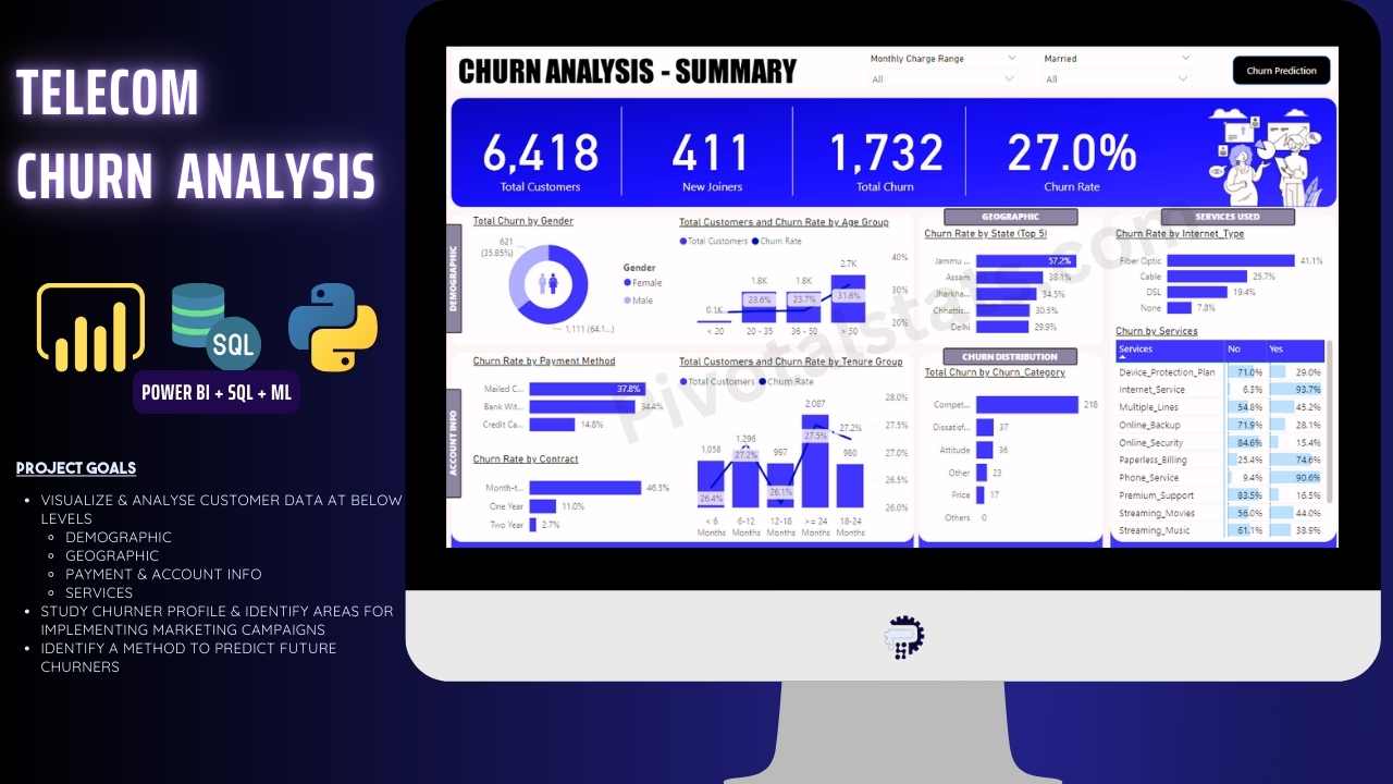
STEP 4 – Power BI Visualization
Summary Page
1. Top Card
a. Total Customers
b. New Joiners
c. Total Churn
d. Churn Rate%
2. Demographic
a. Gender – Churn Rate
b. Age Group – Total Customer & Churn Rate
3. Account Info
a. Payment Method – Churn Rate
b. Contract – Churn Rate
c. Tenure Group – Total Customer & Churn Rate
4. Geographic
a. Top 5 State – Churn Rate
5. Churn Distribution
a. Churn Category – Total Churn
b. Tooltip : Churn Reason – Total Churn
6. Service Used
a. Internet Type – Churn Rate
b. prod_Service >> Services – Status – % RT Sum of Churn Status
Churn Reason Page (Tooltip)
1. Churn Reason – Total Churn
STEP 5 – Predict Customer Churn
For predicting customer churn, we will be using a widely used Machine Learning algorithm called RANDOM FOREST.
What is Random Forest?A random forest is a machine learning algorithm that consists of multiple decision trees. Each decision tree is trained on a random subset of the data and features. The final prediction is made by averaging the predictions (in regression tasks) or taking the majority vote (in classification tasks) from all the trees in the forest. This ensemble approach improves the accuracy and robustness of the model by reducing the risk of overfitting compared to using a single decision tree.
Data Preparation for ML model
Let us first import views in an Excel file.
o Go to Data >> Get Data >> SQL Server Database
o Enter the Server Name & Database name to connect to SQL Server
o Import both vw_ChurnData & vw_JoinData
o Save the file as Prediction_Data
Create Churn Prediction Model – Random Forest
Now we will work with an application called Jupyter Notebook and we will coding our ML model in Python. Easiest way to install both them is to install the ANACONDA Software Package. You can follow the below link to do so:
https://docs.anaconda.com/anaconda/install
Installing Libraries
Open the Anaconda Command Prompt and run below code:
pip install pandas numpy matplotlib seaborn scikit-learn joblib
Open Jupyter Notebook, create a new notebook and write below code:
Importing Libraries & Data Load
import pandas as pd
import numpy as np

import matplotlib.pyplot as plt

import seaborn as sns

from sklearn.model_selection import train_test_split

from sklearn.ensemble

import RandomForestClassifier

from sklearn.metrics import classification_report, confusion_matrix

from sklearn.preprocessing import LabelEncoder

import joblib

# Define the path to the Excel file

file_path = r"C:\yourpath\Prediction_Data.xlsx"


# Define the sheet name to read data from
sheet_name = 'vw_ChurnData'


# Read the data from the specified sheet into a pandas DataFrame
data = pd.read_excel(file_path, sheet_name=sheet_name)


# Display the first few rows of the fetched data
print(data.head())
Data Preprocessing
# Drop columns that won't be used for prediction
data = data.drop(['Customer_ID', 'Churn_Category', 'Churn_Reason'], axis=1)


# List of columns to be label encoded

columns_to_encode = [

    'Gender', 'Married', 'State', 'Value_Deal', 'Phone_Service', 'Multiple_Lines',

    'Internet_Service', 'Internet_Type', 'Online_Security', 'Online_Backup',

    'Device_Protection_Plan', 'Premium_Support', 'Streaming_TV', 'Streaming_Movies',

    'Streaming_Music', 'Unlimited_Data', 'Contract', 'Paperless_Billing',

    'Payment_Method'

]


# Encode categorical variables except the target variable

label_encoders = {}

for column in columns_to_encode:

    label_encoders[column] = LabelEncoder()

    data[column] = label_encoders[column].fit_transform(data[column])


# Manually encode the target variable 'Customer_Status'

data['Customer_Status'] = data['Customer_Status'].map({'Stayed': 0, 'Churned': 1})


# Split data into features and target

X = data.drop('Customer_Status', axis=1)

y = data['Customer_Status']


# Split data into training and testing sets

X_train, X_test, y_train, y_test = train_test_split(X, y, test_size=0.2, random_state=42)
Train Random Forest Model
# Initialize the Random Forest Classifier
rf_model = RandomForestClassifier(n_estimators=100, random_state=42)


# Train the model

rf_model.fit(X_train, y_train)


Evaluate Model

# Make predictions

y_pred = rf_model.predict(X_test)


# Evaluate the model

print("Confusion Matrix:")

print(confusion_matrix(y_test, y_pred))

print("\nClassification Report:")

print(classification_report(y_test, y_pred))


# Feature Selection using Feature Importance

importances = rf_model.feature_importances_

indices = np.argsort(importances)[::-1]


# Plot the feature importances

plt.figure(figsize=(15, 6))

sns.barplot(x=importances[indices], y=X.columns[indices])

plt.title('Feature Importances')

plt.xlabel('Relative Importance')

plt.ylabel('Feature Names')

plt.show()
Use Model for Prediction on New Data
# Define the path to the Joiner Data Excel file
file_path = r"C:\yourpath\Prediction_Data.xlsx"


# Define the sheet name to read data from

sheet_name = 'vw_JoinData'


# Read the data from the specified sheet into a pandas DataFrame

new_data = pd.read_excel(file_path, sheet_name=sheet_name)


# Display the first few rows of the fetched data

print(new_data.head())


# Retain the original DataFrame to preserve unencoded columns

original_data = new_data.copy()


# Retain the Customer_ID column

customer_ids = new_data['Customer_ID']


# Drop columns that won't be used for prediction in the encoded DataFrame

new_data = new_data.drop(['Customer_ID', 'Customer_Status', 'Churn_Category', 'Churn_Reason'], axis=1)


# Encode categorical variables using the saved label encoders

for column in new_data.select_dtypes(include=['object']).columns:

    new_data[column] = label_encoders[column].transform(new_data[column])


# Make predictions

new_predictions = rf_model.predict(new_data)


# Add predictions to the original DataFrame

original_data['Customer_Status_Predicted'] = new_predictions


# Filter the DataFrame to include only records predicted as "Churned"

original_data = original_data[original_data['Customer_Status_Predicted'] == 1]


# Save the results

original_data.to_csv(r"C:\yourpath\Predictions.csv", index=False)
STEP 6 – Power BI Visualization of Predicted Data
Import CSV Data or Load Predicted data in SQL server & connect to server
Create Measures
Count Predicted Churner = COUNT(Predictions[Customer_ID]) + 0
Title Predicted Churners = “COUNT OF PREDICTED CHURNERS : ” & COUNT(Predictions[Customer_ID])
Churn Prediction Page (Using New Predicted Data)
1. Right Side Grid
a. Customer ID
b. Monthly Charge
c. Total Revenue
d. Total Refunds
e. Number of Referrals
2. Demographic
a. Gender – Churn Count
b. Age Group – Churn Count
c. Marital Status – Churn Count
3. Account Info
a. Payment Method – Churn Count
b. Contract – Churn Count
c. Tenure Group – Churn Count
4. Geographic
a. State – Churn Count
That’s it, now you have a comprehensive Power BI dashboard with and Executive Summary to analyze historical data and also a Churn Prediction page to predict future churners. Hope I was able to provide value with this content. Keep following for more content. Cheers!
hi I love this project please coach and kindly help me with the finished work so I can follow along
please provide the dataset of Telecom Churn dataset
Hi, Link is in the description but pasting it here for your reference. Thanks!
https://pivotalstats.com/wp-content/uploads/2024/08/Data-Resources.zip