
Imagine having to sift through a massive dataset, looking for specific insights, and you’re armed only with traditional Excel functions. Intimidating, right? Fortunately, Excel’s Power Pivot, along with the flexibility of DAX, allows you to perform complex calculations akin to COUNTIF and SUMIF but on a grander scale. This enhanced capability is invaluable for professionals dealing with extensive databases.
In this guide, we will unravel how to translate the familiar COUNTIF and SUMIF functions into DAX expressions. By the end, you’ll be equipped with a more advanced understanding of data manipulation in Excel Power Pivot, allowing you to optimize your workflows and deliver insightful analyses effortlessly.
Data Used

Requirement
Create 2 new columns in Power Pivot
- Apply COUNTIF based on City column
- Apply SUMIF based on Profit column based on each City
Understanding the Basics: COUNTIF and SUMIF in Excel
Before diving into DAX, let’s quickly revisit what COUNTIF and SUMIF do in traditional Excel:
What Does COUNTIF Do?
COUNTIF is a simple yet powerful function that counts the number of cells within a range that meet a single condition.
- Syntax:
COUNTIF(range, criteria)
Example: Counting the number of sales transactions above $100.
What Does SUMIF Do?
SUMIF adds the values within a specified range that meet a given condition.
- Syntax:
SUMIF(range, criteria, [sum_range])
Example: Summing total sales for a specific product category.
Transitioning to DAX: COUNTIF Equivalent
In Power Pivot, DAX doesn’t provide direct COUNTIF or SUMIF functions, but it offers a range of functions that allow similar calculations.
Understanding CALCULATE function
The syntax for CALCULATE function is
=Calculate( <expression>, <filter1>, <filter2>,...)
Now if you have not gone through my earlier content on Calculate, let me give you a brief summary. Calculate function lets you evaluate an expression (which usually is some kind of aggregation function), using the tabular data returned by the filter criteria which is also called a calculate modifier.
In today’s topic we will see a type of CALCULATE modifier which is called ALLEXCEPT, let us understand how it works
Understanding ALLEXCEPT function
The syntax for ALLEXCEPT function is
=ALLEXCEPT( <table>, <column>,...)
In simple terms, what ALLEXCEPT does is to instruct the engine to remove filters from everything except the columns mentioned within its parameters.
Now that you have a basic understanding of Calculate function & its modifier, let’s complete the requirement now!
Applying COUNTIF in Power Pivot
- Convert your data into a table and name it as per your choice. I’m going to name it as “ProfitTbl”

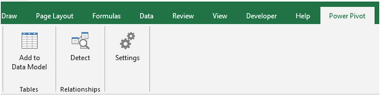
- Select anywhere on the data & go to the Power Pivot tab and click on “Add to Data Model”
- Now you should see the Power Pivot Editor. In this lets create a new calculated column to apply COUNTIF by entering below DAX
=CALCULATE(COUNTA(ProfitTbl[City]),ALLEXCEPT(ProfitTbl,ProfitTbl[City]))
DAX Explanation :
- ALLEXCEPT – This returns a tabular data with filters removed from everything else except for City. Which means for each row it applies a filter for the city present in that row and shows the result
- COUNTA – It’s similar to excel where its counting non-blank values in City column using the tabular data given by ALLEXCEPT
- Finally Calculate evaluates everything together to give the final results
Transitioning to DAX: SUMIF Equivalent
Similar to COUNTIF, we will use the same formula structure but use SUM instead of COUNTA. And use the Profit column.
=CALCULATE(SUM(ProfitTbl[Profit]),ALLEXCEPT(ProfitTbl,ProfitTbl[City]))
Now instead of a column you can use this formula inside a measure as well which will help you to drag these into a pivot table & see the result without duplicate entries like we see here.
Option #2
Transitioning to DAX: COUNTIF Equivalent
In Power Pivot, we can use other functions in combination with CALCULATE which allow similar calculations.
Using CALCULATE and COUNTROWS
In DAX, you achieve COUNTIF functionality by combining the CALCULATE and COUNTROWS functions.
- Example: Counting rows where ‘Sales Amount’ is greater than 100
CountHighSales = CALCULATE(COUNTROWS(Sales), Sales[Sales Amount] > 100)- CALCULATE: Modifies the filter context.
- COUNTROWS: Counts the number of rows in the specified table.
Scenarios in Practice
Imagine managing a retail database where you want to track the number of high-value transactions. Using CALCULATE and COUNTROWS aids in swiftly generating these insights without manual counts.
Transitioning to DAX: SUMIF Equivalent
Here you primarily leverage the CALCULATE and SUM or SUMX functions.
Using CALCULATE and SUM
Here, you’ll use CALCULATE to change the context of the data being summed.
- Example: Calculating the total sales amount over $1000
TotalHighSales = CALCULATE(SUM(Sales[Sales Amount]), Sales[Sales Amount] > 1000)- SUM: Aggregates the values in the specific column.
Using SUMX for More Complex Calculations
For more intricate formulas requiring row-by-row computations, SUMX is beneficial.
- Example: Summing sales values for transactions above $100, considering specific conditions.
ComplexTotalSales = SUMX(FILTER(Sales, Sales[Sales Amount] > 100), Sales[Sales Amount])- SUMX: Iterates through a table and evaluates an expression.
Real-World Application
Consider working with annual budget analysis where specific conditional sums are crucial. By implementing SUMX, complex financial models and projections can be plotted seamlessly.